NLP 201: Text Prepocessing 2 - Vectorization
Natural language processing (NLP) is the ability of a computer program to understand human language
What all tools we need for NLP ?
NLP 101: Text Preprocessing 1 - Cleaning the input
- Tokenization
- Stemming
- Lemmatization
- Stopwords
- Part of Speech Tagging
- Name-Entity Recognition
NLP 201: Text Prepocessing 2 - Basic(Input Text -> Vector)
- One hot Encoding
- BOW
- TF/IDF
- Unigram, Bigram N-grams
NLP 202: Text Prepocessing 3 - Advanced(Input Text -> Vector)
- Word-Embeddings
- Word2Vec, Average Word2Vec
- Glove
NLP 301: Deep Learning - Basic(Modelling)
- RNN
- LSTM
- GRU
NLP 302: Deep Learning - Advanced(Modelling)
- Encoder-Decoder
- Transformers
- Bert
If you are not comfortable with NLP 101 topics.
1. What is Feature Extraction From Text?
Suppose, we have textual data for sentiment analysis, but machine learning models can only understand and work with numbers and not texts. Hence we need to convert our text data into numbers and this process of converting language into numbers is called feature extraction from text, or text vectorization, or text representation.
2. Why do we need it ?
In solving the sentiment analysis problem mentioned above, we require high-quality features to feed into models into NLP pipeline. There's a common adage in machine learning: "garbage in, garbage out." Hence, we need a method to effectively represent our text data as numerical values, ensuring a meaningful semantic representation.
What are techniques for text vectorization ?
- One-hot Encoding
- Bag-of-Words
- N-grams
- TF/IDF
- Some Custom Features
Imagine you have a bag of words containing all the unique words (Vocabulary) in a text. With one hot encoding, you assign each word a unique binary vector, where only one bit is 'hot' (1) and the rest are 'cold' (0). This hot bit represents the presence of that word.
So, You want vector for each word? Great. Now, Let's go back to sentimant task.Suppose you have vocabulary of only 4 words in corpus i.e. you have only 4 words existing in this world and they are: I love my cat.
Now, Before feeding into ML model you need to convert the text I love my cat in vectors of numbers(because algorithms work with numbers and not texts) For that one of the way to to one ohe encode the corpus. we can one-hot encode our corpus like below
I: [1,0,0,0]
love: [0,1,0,0]
my: [0,0,1,0]
cat: [0,0,0,1]
So, when we want to represent the sentence I love my cat, we stack these codes together:
D = [
[1,0,0,0],
[0,1,0,0],
[0,0,1,0],
[0,0,0,1]
]
We have a set of vectorized data ready for our Machine Learning model to understand the sentiment.
Pros
- Intuitive
- Easy to implement
Cons
- Sparse vectors are created
- No fixed size
- Out of Vocabulary Problem
- Can't Capture semantic meaning
i. Using sklearn library.
from sklearn.preprocessing import OneHotEncoder

sentence = "I love my cat"

words = sentence.split() # Convert the sentence into a list of words
words_array = [[word] for word in words] #Convert list of words into a list of lists where each inner list contains a single word


encoder = OneHotEncoder(sparse_output=False)
one_hot_encoded = encoder.fit_transform(words_array)
one_hot_encoded
array([[1., 0., 0., 0.],
[0., 0., 1., 0.],
[0., 0., 0., 1.],
[0., 1., 0., 0.]])ii. Using pandas
import pandas as pd

sentence = "I love my cat"

words = sentence.split()
df = pd.DataFrame(columns=words)
df| I | love | my | cat |
|---|
# Iterate through each word and set corresponding columns to 1
for word in words:
    df[word] = (df.columns == word).astype(int)
    print(df)
    print("----------------")
I love my cat 0 1 NaN NaN NaN 1 0 NaN NaN NaN 2 0 NaN NaN NaN 3 0 NaN NaN NaN ---------------- I love my cat 0 1 0 NaN NaN 1 0 1 NaN NaN 2 0 0 NaN NaN 3 0 0 NaN NaN ---------------- I love my cat 0 1 0 0 NaN 1 0 1 0 NaN 2 0 0 1 NaN 3 0 0 0 NaN ---------------- I love my cat 0 1 0 0 0 1 0 1 0 0 2 0 0 1 0 3 0 0 0 1 ----------------
The Bag of Words model represents text by counting word occurrences i.e how many time a word appeared in corpus, disregarding grammar and order.
Note: It performs good on tasks like sentiment analysis and classification but may lose context and meaning.
Steps
Step 1: Tokenize the corpus:
Let's have a corpus with vocabulary, I love my cat oscar a lot. Note that This corpus has 7 length vocabulary.
Let's go back to I love my cat example. We will make a bag of word for this with respect to above vocabulary. After tokenization, break the sentence into words as:
"I", "love", "my", "cat"
Step 2:Vocabulary Creation
Create a list of unique words in the phrase: ["I", "love", "my", "cat"]
Step 3: Counting Word Occurrences
Count how many times each word appears:
- I: 1 time
- love: 1 time
- my: 1 time
- cat: 1 time
- Oscar: 0 time
- a: 0 time
- lot: 0 time
Step 4: Vector Representation
Since each word in I love my cat appears once and Oscar a lot doesn't appear in the example, the Bag of Words vector would look like:
| I | love | my | cat | Oscar | a | lot |
|---|---|---|---|---|---|---|
| 1 | 1 | 1 | 1 | 0 | 0 | 0 |
So the vector of BOW will be:
Note that, the vocabulary was of 7 length, the BOW vector are also are 7 length
Lets see how a data frame for BOW is created
Consider same corpus as above with vocabulary, I love my cat oscar a lot.
| Sno | Sentence | I | love | my | cat | Oscar | a | lot |
|---|---|---|---|---|---|---|---|---|
| 1 | I love my cat Oscar a lot | 1 | 1 | 1 | 1 | 1 | 1 | 1 |
| 2 | I love Oscar a lot | 1 | 1 | 0 | 0 | 1 | 1 | 1 |
| 3 | I love my cat | 1 | 1 | 1 | 1 | 0 | 0 | 0 |
| 4 | Oscar my cat oscar | 0 | 0 | 0 | 1 | 2 | 0 | 0 |
| 5 | love cat love cat cat | 0 | 2 | 0 | 3 | 0 | 0 | 0 |
| 6 | love cat my love cat | 0 | 2 | 1 | 0 | 0 | 0 | 0 |
In above dataframe for example 5, love cat love cat cat, The appearance of words are as:
| Word | Count |
|---|---|
| I | 0 |
| love | 2 |
| my | 0 |
| cat | 3 |
| Oscar | 0 |
| a | 0 |
| lot | 0 |
Hence, the Bag of Vector for this will be:
Let's, learn how create BOW vectors in python
In the dataframe above, sentiments have been randomly assigned.
data = {
    'Sentence': [
        'I love my cat Oscar a lot',
        'I love Oscar a lot',
        'I love my cat',
        'Oscar my cat oscar',
        'love cat love cat cat',
        'love cat my love cat'
    ],
    'Sentiment': [
        'positive',
        'positive',
        'positive',
        'neutral',
        'neutral',
        'neutral'
    ]
}

df = pd.DataFrame(data)

df| Sentence | Sentiment | |
|---|---|---|
| 0 | I love my cat Oscar a lot | positive |
| 1 | I love Oscar a lot | positive |
| 2 | I love my cat | positive |
| 3 | Oscar my cat oscar | neutral |
| 4 | love cat love cat cat | neutral |
| 5 | love cat my love cat | neutral |
Note: This type of dataset is commonly used for sentiment classification data.
from sklearn.feature_extraction.text import CountVectorizer

bow_vectorizer = CountVectorizer()
bow_vectors = bow_vectorizer.fit_transform(df['Sentence'])
We can get the for a vector index represent what word using vocabulary_ method
bow_vectorizer.vocabulary_{'love': 2, 'my': 3, 'cat': 0, 'oscar': 4, 'lot': 1}Note: We originally had a vocabulary of 7 words, but after using CountVectorizer, our vocabulary was reduced to 5 words. This happened because CountVectorizer remove words that are stop words.
Let view the bow_vectors
bow_vectors<6x5 sparse matrix of type '<class 'numpy.int64'>' with 19 stored elements in Compressed Sparse Row format>
Tt is currently an compressed as object. To convert this object into matrix.
Use toarray() method
print(bow_vectors.toarray())[[1 1 1 1 1] [0 1 1 0 1] [1 0 1 1 0] [1 0 0 1 2] [3 0 2 0 0] [2 0 2 1 0]]
Note: We can also get bow vector for individual sentences using indexing.
print(bow_vectors[0].toarray())[[1 1 1 1 1]]
print(bow_vectors[1].toarray())[[0 1 1 0 1]]
Let transform a new sentence love my dog oscar love oscar oscar
# {'love': 2, 'my': 3, 'cat': 0, 'oscar': 4, 'lot': 1} --------------> this is the hashing for vectors
document = "love my dog oscar love oscar oscar"
bow_vectorizer.transform([document]).toarray()
array([[0, 0, 2, 1, 3]])
Note:
- The vector was created using the frequency of love, my, and oscar. The word dog was ignored because it was not present during training. This demonstrates how the Bag of Words (BoW) model handles out-of-vocabulary words in the data(simply by ignoring).
Consider exploring WordVectorizer module in sklearn
Problems in one hot encoding solved by Bag of Word
1. Fix word size, no. of words in document doesn't matter.
Consider a corpus with vocabulary "I love my cat". Then we can vectorize below documents as
I love my cat ------> [1, 1, 1, 1]
I love cat ------------->[1, 1, 0, 1]
Note that, both document will have same size BOW vector.
2. It also handle out of vocabulary error in new sentence by simply ignoring the word while creating bag of word vector.
Cons in Bow
1. Ignoring the OOV word in new sentence might lose the meaning in sentence.
For example:
We have
- I love cat ------------->[1, 1, 0, 1]
Now, if we convert the sententce I don't love cat into BOW, and since the word don't was not there during training. Then
- I don't love cat ------------->[1, 1, 0, 1]
Both I love cat and I don't love cat will have same vector in that case, which is wrong because both sentence have opposite meaning and infromation which don't could provide is lost.
2. Despite the representation as Bag-of-Words (BOW), vectors remain sparse. When the vocabulary is extensive, even after vectorizing a sentence, numerous elements in the vector will retain a value of 0.
3. Not Considering ordering of Sentence is an issue
The Bag of Words (BoW) model simply counts how often each word shows up in a corpus, without caring about grammar or the order of words. Then, it convert each document in corpus into a list showing how many times each word appears.
Earlier in one-hot encoding or bag-of-words, the vocabulary consisted of single words, and the problem with that was we could not exploit the ordering in the sentence. We were not able to capture the semantic meaning in sentences because ordering is very important in language.
We solve this problem with N-grams, where the vocabulary consists of sequences of N words.
For example:
The tokenization for I love my cat oscar a lot using bi-gram will be: I love / love my /my cat/ cat oscar/ oscar a/ alot. Its like sliding window of size 2.
Note: I have not considered existance of stopwords.
| Sentence | I love | love my | my cat | cat oscar | oscar a | a lot | Ngram vector |
|---|---|---|---|---|---|---|---|
| I love my cat oscar a lot | 1 | 1 | 1 | 1 | 1 | 1 | [1, 1, 1, 1, 1, 1] |
| I love cat a lot | 1 | 0 | 0 | 0 | 0 | 1 | [1, 0, 0, 0, 0, 1] |
| I love my cat oscar | 1 | 1 | 1 | 1 | 0 | 0 | [1, 1, 1, 1, 0, 0] |
Note that: Bag of Words is a special case of bag of N-grams i.e it is unigram
In sklearn's CountVectorizer() pass
- ngram_range = (1,1): only BOW or unigrams
- ngram_range = (2,2): only bi-gram
- ngram_range = (1,2): both uni-gram/BOW
- ngram_range = (1,3): uni-gram/BOW and bigrams, and trigrams
- ngram_range = (2,3): both bi-grams, and trigrams
- ngram_range = (2,3): only tri-grams
Pros and Cons of N-grams
| Pros | Cons |
|---|---|
| 1. Captures local context and dependencies. | 1. Increased dimensionality of vocabulary with increase N |
| 2. Captures some semantic meaning | 2. Data sparsity issues with higher-order N-grams. |
| information. | 3. No solution for handling out of vocabulary OOV error |
| 3. Can handle variable-length sequences. |
|
from sklearn.feature_extraction.text import CountVectorizer

bi_vectorizer = CountVectorizer(ngram_range=(2,2))

document = ["I love my cat oscar a lot"]

bi_vectorizer.fit(document) # it take document in a list of sentences, don't feed sentences directly.

bi_vectorizer.vocabulary_
{'love my': 1, 'my cat': 2, 'cat oscar': 0, 'oscar lot': 3}Note:
- love my: 1: This indicates that the bigram "love my" is assigned the index 1.
- my cat: 2: This indicates that the bigram "my cat" is assigned the index 2.
- cat oscar: 0: This indicates that the bigram "cat oscar" is assigned the index 0.
- oscar lot: 3: This indicates that the bigram "oscar lot" is assigned the index 3.
bi_vectorizer.transform(["I love my cat oscar a lot"]).toarray()array([[1, 1, 1, 1]])
bi_vectorizer.transform(["I love cat a lot"]).toarray()array([[0, 0, 0, 0]])
bi_vectorizer.transform(["I love my cat a lot"]).toarray()array([[0, 1, 1, 0]])
Lets see how N-gram works with multiple sentences.
data = {
    'Sentence': [
        'I love my cat Oscar a lot',
        'I love Oscar a lot',
        'I love my cat',
        'Oscar my cat oscar',
        'love cat love cat cat',
        'love cat my love cat'
    ],
    'Sentiment': [
        'positive',
        'positive',
        'positive',
        'neutral',
        'neutral',
        'neutral'
    ]
}

df = pd.DataFrame(data)

print(df)
Sentence Sentiment 0 I love my cat Oscar a lot positive 1 I love Oscar a lot positive 2 I love my cat positive 3 Oscar my cat oscar neutral 4 love cat love cat cat neutral 5 love cat my love cat neutral
bigram_vectorizer = CountVectorizer(ngram_range=(2,2))

bigram_vectorizer.fit_transform(df['Sentence'])
<6x11 sparse matrix of type '<class 'numpy.int64'>' with 17 stored elements in Compressed Sparse Row format>
bigram_vectorizer.vocabulary_{'love my': 5,
'my cat': 7,
'cat oscar': 3,
'oscar lot': 9,
'love oscar': 6,
'oscar my': 10,
'love cat': 4,
'cat love': 1,
'cat cat': 0,
'cat my': 2,
'my love': 8}bigram_vectorizer.transform(['I love my cat oscar a lot']).toarray()array([[0, 0, 0, 1, 0, 1, 0, 1, 0, 1, 0]])
Problem with one-hot encoding, Bag of words, N-grams:
All of these three text representation techniques assign equal importance to all the tokens. They assign 0 if a word is absent in the sentence, and 1 if the word is present.
TF-IDF solves this problem by assigning different values to different words.
TF-IDF assigns weights to words based on how frequently they appear in a document compared to their frequency across all documents in the dataset.
It uses two measures to calcuate importance:
- Term Frequency (TF)
- Inverse Document Frequency (IDF)

Logic for TF-IDF is simple:
It assigns higher weightage to those word in document whose frequency is more in that particular document but are rare across corpus.
| Pros | Cons |
|---|---|
| Weighted Representation of words | High dimensional vectors |
| Robustness to Stop Words | Lack of semantic meaning |
| Interpretability | Produces sparse vectors |
| Widely Used | Can't handle OOV words |
data = {
    'Sentence': [
        'I love my cat Oscar a lot',
        'I love Oscar a lot',
        'I love my cat',
        'Oscar my cat oscar',
        'love cat love cat cat',
        'love cat my love cat'
    ],
    'Sentiment': [
        'positive',
        'positive',
        'positive',
        'neutral',
        'neutral',
        'neutral'
    ]
}

df = pd.DataFrame(data)

print(df)
Sentence Sentiment 0 I love my cat Oscar a lot positive 1 I love Oscar a lot positive 2 I love my cat positive 3 Oscar my cat oscar neutral 4 love cat love cat cat neutral 5 love cat my love cat neutral
from sklearn.feature_extraction.text import TfidfVectorizer

tfidf_vectorizer = TfidfVectorizer()

tfidf_vectorizer.fit_transform(df['Sentence']).toarray()
array([[0.35970394, 0.57573099, 0.35970394, 0.41652649, 0.48607166],
[0. , 0.68955073, 0.43081598, 0. , 0.58216611],
[0.54710234, 0. , 0.54710234, 0.63352827, 0. ],
[0.32199391, 0. , 0. , 0.3728594 , 0.87022743],
[0.83205029, 0. , 0.5547002 , 0. , 0. ],
[0.65438863, 0. , 0.65438863, 0.37888131, 0. ]])Note that
IDF values are consistent across the entire corpus, unlike TF, which varies from document to document. Let's get out the IDF vector for each token. IDF measures how important a word is within a collection of documents.
print(tfidf_vectorizer.idf_)
print(tfidf_vectorizer.get_feature_names_out())
[1.15415068 1.84729786 1.15415068 1.33647224 1.55961579] ['cat' 'lot' 'love' 'my' 'oscar']
Interpretation:
- The token cat has an IDF value of approximately 1.154.
- The token lot has an IDF value of approximately 1.847.
- The token love has an IDF value of approximately 1.154.
- The token my has an IDF value of approximately 1.336.
- The token oscar has an IDF value of approximately 1.560.
Here, these IDF values help us understand the significance of each token across the corpus. Tokens like "lot" and "oscar" have higher IDF values, suggesting they are relatively more unique or rare compared to tokens like "cat" and "love," which have lower IDF values, indicating they are more common across the corpus.
Remark
You'll get bigger IDF values in sklearn's TF-IDF because they have a little different Implementation of TF-IDF than original TF-IDF
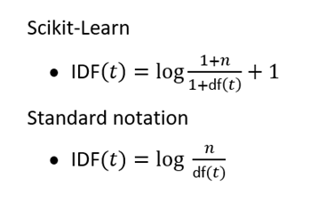
Reasoning
Addition of 1 to numerator and denominator: Ensures non-zero IDF for terms with zero document frequency, avoiding division by zero errors.
Addition of 1 orginal TF-IDF : Prevents terms in all documents from having zero IDF, ensuring no term is disregarded entirely in TF-IDF calculation.
Imagine you're looking at two words: cat and dog, in a bunch of documents.
Let's say
- dog appears in 500 out of 1,000 documents
- cat only shows up in 10 of 1000 documents.
If we calculate IDF without log, we get:
Without logarithms, the IDF values for dog and cat are very different: dog has an IDF of 2, while cat has an IDF of 100. This discrepancy highlights that cat is considered much rarer across the document corpus compared to dog.
The unbalanced representation of IDF values can skew TF-IDF scores, favoring terms like cat that are rare across documents. This dominance of rare terms like cat can make the importance of more frequent terms like cat almost neighligible in TF-IDF.
Taking log helps to mitigate this imbalance by scaling down the impact of exteme IDF values.